What Is Swept Path Analysis? Geometry, Worked Example and How to Do One

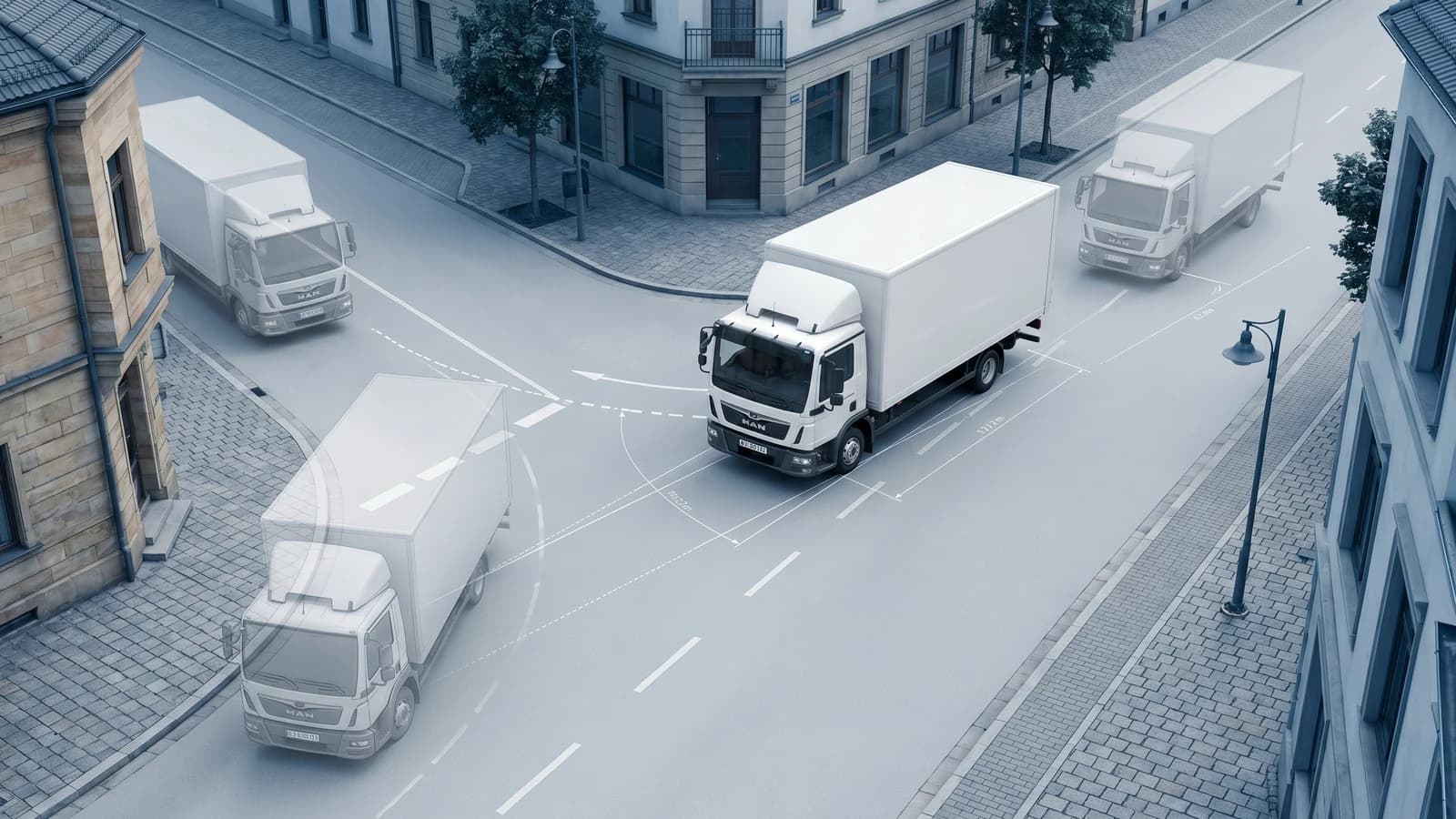
Swept path analysis is the geometric calculation of the exact area a vehicle occupies while turning, accounting for off-tracking: the rear wheels don't follow the front wheels, they cut inside the curve, so the space the vehicle sweeps through is wider than the vehicle itself. Civil engineers use it to predict that swept area exactly, so a fire truck reaches a hydrant, a delivery van clears a bollard, and a refuse vehicle backs out of a dead end without climbing the kerb.
This guide explains what swept path analysis is and who uses it, derives the geometry from first principles, walks through a worked pen-and-paper example, and shows how to do a swept path analysis step by step. No specific country's regulations are required; the underlying physics applies everywhere.
TL;DR. In a steady-state turn, a rigid vehicle's swept envelope is bounded by just two reference paths: the outer-front corner (outer edge) and the inner-rear wheel (inner edge: wheel, not corner). A third path, the outer-rear corner, defines the tail swing at the start of every turn: a brief outboard swing of the rear caused by the rear overhang, regardless of how fast the steering input is applied. All three can be computed from five numbers: length, width, wheelbase, front overhang, rear overhang. Worked example below.
What is swept path analysis?
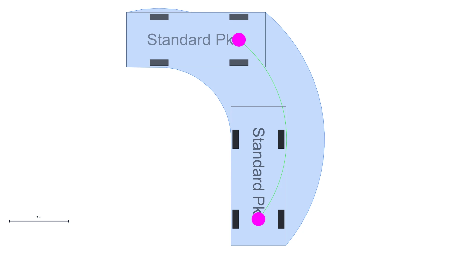
Swept path analysis (also called vehicle tracking or off-tracking analysis; the method is compared with the product of that name in PathSweeper vs Autodesk Vehicle Tracking) computes a vehicle's swept path: the area the vehicle physically occupies while turning, the union of every position the vehicle body passes through during the manoeuvre.
You need it because:
- An intersection, a fire-truck turning bay, a parking-garage ramp or an alleyway is only as useful as the vehicles that can fit through it.
- The geometric envelope is bigger than the bare vehicle width, and the difference matters: a typical lorry occupies a footprint about 1.5× its own width during a sharp turn.
- Without the envelope, you can't verify clearance from kerbs, walls, columns, parked cars, or fire hydrants.
Who uses swept path analysis, and when?
Swept path analysis sits at the intersection of several professions. Highway and traffic engineers run it on junctions, roundabouts and bus stops. Architects and site planners run it on driveways, parking layouts and delivery yards. Developers and logistics operators run it to prove a site works before committing to it. The typical scenarios:
- Junctions and roundabouts: verifying that the design vehicle can make every permitted turning movement without crossing into opposing lanes or mounting splitter islands.
- Parking and garage ramps: checking that cars actually reach the stalls, and that ramps and helix curves work at their regulated minimum radii; the worked example below is exactly this car-scale geometry.
- Loading bays and delivery zones: the classic commercial case, usually with a rigid truck or semi-trailer reversing to a dock.
- Dead-end streets and turning bays: refuse vehicles must turn without long reversing; the layouts are covered in the turning bay design guide.
- Fire and emergency access: access-road checks for fire apparatus; see the fire truck access guide.
- Construction routes and abnormal loads: one-off proofs that a crane, low-loader or oversized transport can reach the site.
When is it required, rather than merely wise? That depends on jurisdiction, but the pattern is consistent: local authorities frequently ask for a swept path check as part of a planning or building application whenever drivability of an access, turning area or delivery zone isn't obvious from the drawing. It's routinely commissioned as a drawing annex rather than a standalone report.
The geometry: why the rear wheel cuts the corner (Ackermann steering, in plain words)
Rudolph Ackermann's 1817 patent describes how a steered vehicle's wheels move during a turn. Its central insight:
During a turn, every wheel of the vehicle traces a circle around a single shared centre point, the instantaneous centre of rotation (ICR).
The ICR sits on the extension of the rear axle (because the rear wheels don't steer, their rolling direction is fixed perpendicular to the axle). The front wheels are angled exactly so their perpendicular lines also pass through this same ICR. That alignment (front wheels turning to slightly different angles so their lines meet at one point) is what we call Ackermann geometry.
The consequence: every point on the vehicle traces its own circle around the ICR. The largest circle is traced by the outer-front corner of the body. Because of the front overhang, the corner sits further from the ICR than the outer-front wheel, and it defines the outer edge of the swept envelope. The smallest circle is traced by the inner-rear wheel at the axle, which defines the inner edge. The body sweeps the annular region between these two paths.
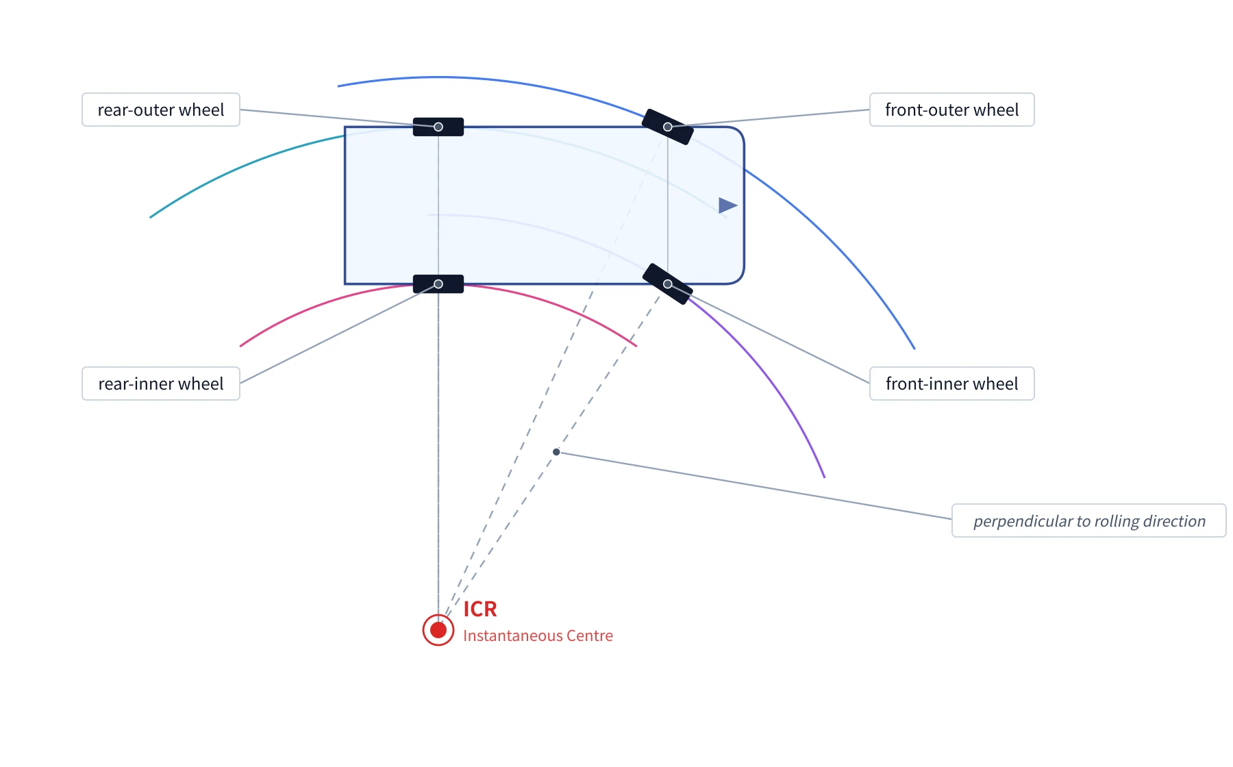
The math, if you want it. With the ICR on the extension of the rear axle, let R be the distance from ICR to the centre of the rear axle (the rear-axle radius). Then the inner-rear-wheel radius is R − w/2 and the outer-front-corner radius is √[(R + w/2)² + (wb + fo)²], where w is vehicle width, wb is wheelbase, and fo is front overhang. Knowing any one of these radii pins down all the others.
The reference paths
Three reference paths cover the envelope. Two bound it during the steady-state portion of the turn; one more, the outer-rear corner, defines a brief outboard sweep at the start of every manoeuvre.
Steady-state bounds
| Reference | What traces it | Role |
|---|---|---|
| Outer-front-corner path | The outer corner of the front bumper | The outer edge of the envelope. Checked against kerbs, walls, lamp posts on the outside of the curve. |
| Inner-rear-wheel path | The inner rear wheel at the axle level | The inner edge of the envelope. Wheel, not corner; the wheel sits inboard of the body corner, so the wheel always defines the inner clearance. |
In pure circular motion these two paths alone fully describe where the vehicle is. Everything else on the body sits inside the annulus between them.
Tail swing
| Reference | When it matters |
|---|---|
| Outer-rear-corner path | At the start of every turn the rear of the body briefly swings outboard of the straight-ahead heading: tail swing. This is a geometric consequence of the rear overhang and happens regardless of how fast the steering input is applied; even with an instantaneous steering change the rear corner enters its circular path from a position behind the front, so its swept arc reaches outside the steady-state envelope at the moment of entry. Once the vehicle is in steady circular motion the outer-rear corner sits on a smaller radius than the outer-front corner and lies inside the envelope. Tail swing is treated as its own design check in many regulations (see for example Australia's NHVR PBS standard). |
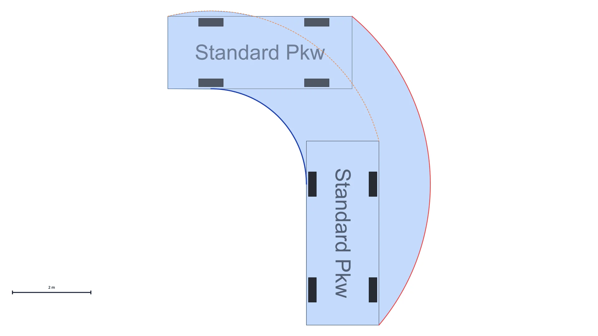
The single most common mistake, even in some published work, is to assume the inner rear corner of the body defines the inner edge of the envelope. It doesn't. The corner is wider than the wheel, so its path lies outboard of the wheel's path. The wheel, not the corner, sets the inner clearance.
The five numbers you need
For a non-articulated vehicle (passenger car, van, two-axle truck, bus), five dimensions fully describe the geometry of a constant-radius turn:
| Symbol | Name | Description |
|---|---|---|
| L | Length | Total vehicle length, bumper to bumper |
| w | Width | Total vehicle width, including mirrors if relevant |
| wb | Wheelbase | Distance between front and rear axle |
| fo | Front overhang | Front bumper to front axle |
| ro | Rear overhang | Rear axle to rear bumper |
The minimum turning radius (the smallest circle the vehicle can drive) is fixed by the maximum steering angle of the front wheels, which is a property of the vehicle itself. Commercial-vehicle datasheets often list it directly as the outer turning radius (front-outer-corner). Passenger-car brochures usually give a turning circle diameter instead, which has to be halved.
Read the exact wording, because three different circles are in circulation:
| Figure | Measured at | Usable as a front-corner radius |
|---|---|---|
| Turning circle (DIN 70020: the parts of the vehicle protruding furthest to the outside of the curve), sometimes labelled wall-to-wall | body | Yes, halve the diameter |
| Kerb-to-kerb | outer sidewall of the outer front tyre | No, too small |
| Track circle (Spurkreis) | centre of the outer front wheel | No, smaller still |
The front outer corner sits further out than any wheel because of the front overhang, by roughly half a metre in radius on a passenger car. Using either wheel-based figure as a front-corner radius makes the swept path come out too narrow, so the result looks more optimistic than reality.
Swept path analysis example: a typical passenger car, worked by hand
Let's work out a car swept path by hand: the four reference paths of a standard passenger car making its tightest right-hand turn. Dimensions roughly matching a real-world VW Golf or BMW 3-series:
| Length L | 4.70 m |
| Width w | 1.85 m |
| Wheelbase wb | 2.70 m |
| Front overhang fo | 0.90 m |
| Rear overhang ro | 1.10 m |
| Outer turning radius R_out | 5.60 m |
The outer turning radius of 5.60 m is the path of the outer front corner, measured from the ICR. We work backwards from there.
Step 1: Find the rear-axle radius
The outer front corner sits at distance (wb + fo) = 3.60 m forward of the rear axle, and w/2 = 0.925 m outboard of the rear-axle centre. By Pythagoras:
R_out² = (R_rear + w/2)² + (wb + fo)²
5.60² = (R_rear + 0.925)² + 3.60²
31.36 = (R_rear + 0.925)² + 12.96
(R_rear + 0.925)² = 18.40
R_rear + 0.925 = 4.29
R_rear = 3.36 m
So the centre of the rear axle traces a circle of radius 3.36 m around the ICR.
Step 2: Inner rear wheel
The inner rear wheel is half a vehicle width inboard of the rear-axle centre:
R_inner_wheel = R_rear − w/2 = 3.36 − 0.925 = 2.44 m
Step 3: Outer rear corner
The outer rear corner sits ro = 1.10 m behind the rear axle and w/2 = 0.925 m outboard. Its distance from the ICR is:
R_outer_rear = √[(R_rear + w/2)² + ro²] = √[4.29² + 1.10²] = 4.43 m
Step 4: Inner front corner
The inner front corner sits (wb + fo) = 3.60 m forward of the rear axle and w/2 = 0.925 m inboard. Its distance from the ICR is:
R_inner_front = √[(R_rear − w/2)² + (wb + fo)²] = √[2.44² + 3.60²] = 4.35 m
Result
| Reference | Radius |
|---|---|
| Outer-front corner | 5.60 m ← given |
| Outer-rear corner | 4.43 m |
| Inner-front corner | 4.35 m |
| Inner-rear wheel | 2.44 m |
The swept envelope is the annular region between the inner-rear-wheel circle (2.44 m) and the outer-front-corner circle (5.60 m). For this passenger car, that's a band 3.16 m wide, roughly 1.7× the vehicle's own width.
Note that the outer-rear corner (4.43 m) and the inner-front corner (4.35 m) both sit inside this annulus in steady-state circular motion. The outer-rear corner becomes limiting at the start of the turn (tail swing); the inner-front corner is interior throughout for this passenger-car geometry.
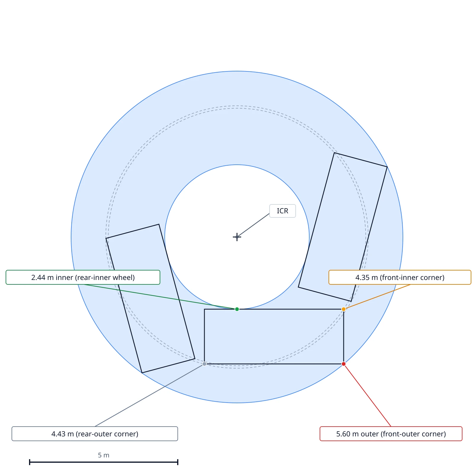
Why we used a 90° turn assumption. This calculation gives you the radii of the full circles each reference traces. A real intersection turn typically uses only an arc of those circles (the steering angle is held constant briefly, then released). Software tracks the actual arc swept; the radii here tell you how wide it gets at maximum input.
Real-world considerations beyond the textbook model
The Ackermann low-speed model is exact in principle, but real vehicles deviate from it for three reasons. Most regulatory checks ignore these because they're designed around low-speed manoeuvres, but it's worth knowing where the model breaks.
1. Heading changes are not instantaneous
The model assumes the steering input changes the front-wheel angle immediately. In reality, the driver turns the steering wheel over half a second to two seconds, and during that time the actual swept path is a transition curve, not a circular arc. For passenger cars at planning scales this is negligible; the transition is visible only at sub-metre resolution. For long articulated vehicles (semi-trailers, B-doubles), the transition matters and software typically models it explicitly, which is what PathSweeper's rate-limited steering mode does.
2. At higher speed, the rear wheels track outboard
Above roughly 30 km/h, tyre slip becomes significant. The rear wheels develop a small slip angle (typically 1–3°) that pushes the rear of the vehicle outboard of its kinematic path. This widens the outer envelope, sometimes by 0.5 m for a lorry. For driveways, parking, fire access and most urban planning, low-speed kinematics is correct. For motorway entry/exit ramps, racetracks and crash reconstruction, you need a dynamic model.
3. Articulated vehicles add a second envelope
A semi-trailer is two rigid bodies connected by a hinge. Each follows its own Ackermann geometry around the same ICR, but the trailer's rear axle traces a smaller circle than the towing vehicle's. This is the famous off-tracking of a long lorry: the trailer cuts the corner. Articulated buses, B-trains, and double-trailer combinations stack this effect; the rearmost trailer can cut the corner by several metres on a sharp turn.
There's a second subtlety unique to articulated geometry. The rigid-vehicle shortcut of "track only the body corners and connect the dots" no longer gives the exact envelope, because the trailer's hinge point itself moves along the tractor's path while the trailer rotates around it. At certain phases of the turn the inner edge of the trailer's swept area is defined not by the trailer's corner but by a point along the trailer's side, typically near the rear axle group. Production tools like AutoTURN, Vehicle Tracking and AutoPATH handle this by sampling many points along the entire vehicle perimeter at every timestep and taking the union, rather than relying on four corners. PathSweeper computes its articulated envelope the same way, a full-perimeter sampling-and-union pass, so it captures that inner-side point rather than the four-corner shortcut that would underestimate the true envelope on sharp turns. How the individual combination types differ, from drawbar trailer to articulated bus, is set out in the post on articulated vehicle swept paths.
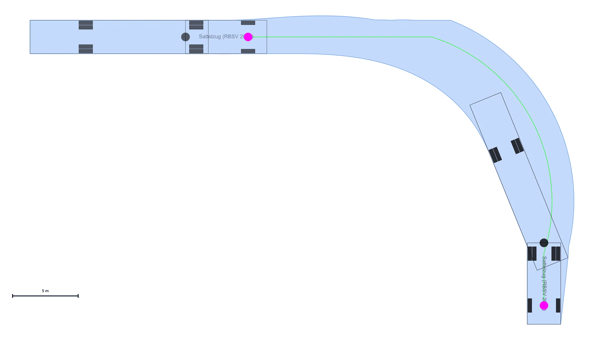
For these, hand calculation is impractical and software is essentially required.
How to do a swept path analysis, step by step
Whatever tool you use (CAD plugin, browser tool, or the pen-and-paper method above for simple cases; the field is surveyed in our swept path software comparison), the procedure is the same:
- Choose the design vehicle. Not the vehicle you happen to own: the largest vehicle that must regularly use the space, or the one your authority specifies. National design-vehicle catalogues exist precisely for this step (see the country guides below).
- Get a to-scale base plan. A site plan, cadastral extract or measured survey showing every fixed obstacle: kerbs, columns, walls, trees, parking stalls. Without a reliable scale, the whole analysis is decorative.
- Define the manoeuvre. Each real movement separately: entry, exit, each direction of travel, and reverse manoeuvres (docking, backing out) as their own checks.
- Trace the path. Draw the trajectory the driver would actually steer, including the transition into the turn, not an idealised circular arc.
- Generate the envelope. Compute the swept envelope along the path with a kinematic model. For articulated vehicles the tractor and trailer must be modelled separately around their hinge.
- Check clearances. Compare the envelope against the obstacles on the plan, with a safety margin on all sides; authorities commonly expect a visible buffer rather than a tangent hit.
- Document the result. Scale, named design vehicle, direction arrows, the envelope itself and the margin, on the drawing; export to PDF, or as DXF and DWG straight into the CAD plan, as the submission requires.
Steps 4–6 are where hand methods run out: a real trajectory isn't a constant-radius circle, and the envelope must be integrated along it. That's the part software automates; the free in-browser route is to draw the path directly in PathSweeper over your uploaded plan.
What a swept path diagram must show
Step 7 deserves its own word, because the swept path diagram (the drawing itself) is what a reviewer actually sees, and diagrams get rejected for missing information more often than for bad geometry. A submittable swept path drawing shows:
- Scale, stated and drawn (a scale bar survives PDF resizing; a bare ratio doesn't)
- The design vehicle, named on the sheet with its key dimensions
- The driven path with direction arrows, so the reviewer can distinguish forward from reverse
- The swept envelope itself, visually distinct from the vehicle outline
- The clearance margin to kerbs, walls, columns and parked vehicles
- One movement per sheet where several manoeuvres would overlap illegibly
FIG 1 and FIG 4 above are exactly this kind of diagram: envelope, reference paths and dimensions on one drawing. If your authority provides its own drawing standard, it will typically ask for these same elements plus a title block. For the click-by-click route to such a sheet, see how to create a swept path diagram without CAD.
From paper to PathSweeper
The numbers above show that even a single passenger car needs five inputs and four output radii. A real planning task is rarely a single constant-radius circle; it's a sequence of turns, of varying radii, possibly with reverse manoeuvres, against a real site plan with kerbs, parked cars, columns and trees. Doing all of that by hand is a project in itself.
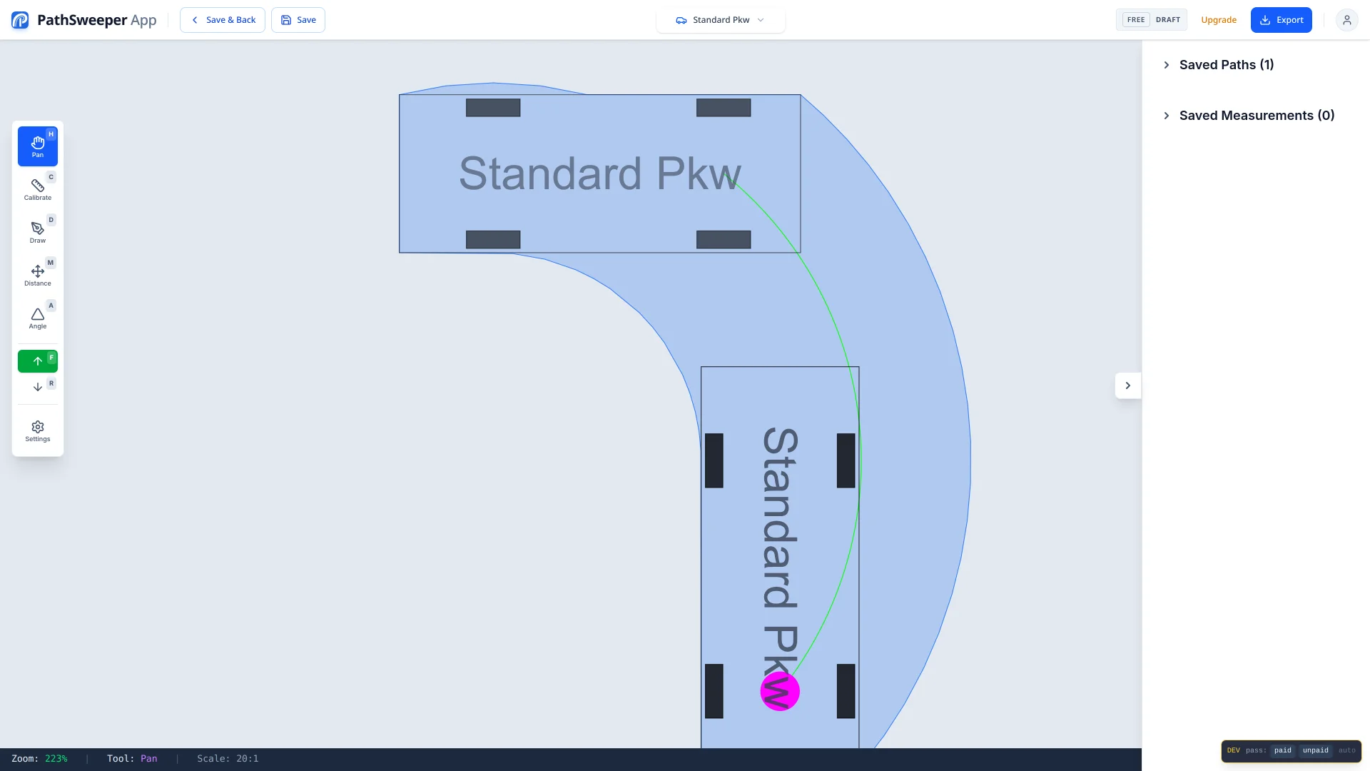
PathSweeper computes all of this in real time as you draw the trajectory, against your uploaded site plan. The same underlying geometry, but in seconds rather than an afternoon, including articulated vehicles, reverse manoeuvres, and full-perimeter clearance reporting. How closely that engine agrees with AutoTURN Online on the 13 German design vehicles is documented, per vehicle, in the engine validation report.
Country-specific design vehicles
The geometry is universal, but the vehicles you check against are usually mandated by national or regional standards. Each country specifies a list of design vehicles with concrete dimensions you must use for regulated submissions:
- Germany: RBSV 2020 design vehicles
- USA: AASHTO Green Book design vehicles
- United Kingdom: DMRB design vehicles
- Australia: Austroads design vehicles
Each of those guides lists what's free to use and where the official publications fit in. Where a project names no catalogue at all, the German statutory turning ring, the BO-Kraftkreis, is a free worst-case baseline that every road-legal vehicle has to fit into.
PathSweeper runs in your browser, no install required. The full swept-path engine, true Ackermann steering, full articulation, national design-vehicle libraries and dimensioned DXF and DWG export are live today; the four generic standard vehicles (car, van, truck, bus) are free to use, and the national libraries unlock with a Project Pass.